The Discrete Fourier Transform: Amplitude scaling between the time and frequency domains

Introduction
(TLDR) Amplitude scaling in the time and frequency domains
(In detail) Amplitude scaling in the time and frequency domains
- 3.1 Introduction
- 3.2 DFT of a cosine signal that is periodic in $N$
- 3.3 Summary
Amplitude scaling for periodic signals with a constant phase shift
Power spectra
Further reading

1 Introduction

Consider a real valued discrete time signal $x[n]$ defined as

(1) $\begin{align*} x[n] = A_1 \cos (2 \pi n k_{1}/N) \end{align*}$

for amplitude $A_1$ , frequency $k_1$ (assumed to be an integer), total number of samples $N$ (also an integer), and integer time index $n = 0, 1, 2, ... , N-1$ .

Is there a single-sided frequency domain representation of $x[n]$ where the signal magnitude, $A_1$ , can be read off at the appropriate bin frequency?

The short answer is provided below. More detail and proofs are provided later on.

2 (TLDR) Amplitude scaling in the time and frequency domains

2.1 Scaling concepts

The DFT of the signal given by equation 1, calculated in the conventional way as used in Matlab and Python, is defined as

(2) $\begin{align*} X[k] &= \sum_{n=0}^{N-1} x[n] e^{-2\pi i k n/N}, \hspace{0.5cm} k = 0, 1, 2, ... , N-1 \end{align*}$

resulting in a set of $N$ complex amplitudes $X[k]$ (note that, as usual, expressing the DFT in terms of other frequency variables is also possible; we’ll stick with the representation in equation 2 as it’s notationally simplest).

Comments:

We assume a rectangular window has been used to obtain the $N$ samples within $x[n]$ , and so omit it from the definition.
As we’ll see later on, implementing the DFT via equation 2 causes the complex amplitude entries to be scaled by a factor $N$ . However, since we know the scaling, the units of $X[k]$ can be re-scaled so as to `match’ those of $x[n]$ . We will called this re-scaled spectrum $X_{S}[k]$ .
Rescaling DFT amplitudes is useful where preserving the physical units of the time domain signal, e.g., sound pressure or surface velocity, will be of relevance in the frequency domain analysis.
The spectrum structure of $X[k]$ is slightly different depending on whether $N$ is even or odd. Therefore, the exact scaling calculations are listed separately in the next two sub-sections.

2.2 DFT scaling computations: N is even

If $N$ is even we calculate $X_{S}[k]$ by taking a single-sided view of the spectrum $X[k]$ , running from $k = 0:\frac{N}{2}$ (i.e., up to the Nyquist limit), and scaling the complex amplitudes according to

(3) $\begin{align*} X_{S}[k]= \begin{cases} \left (\frac{1}{N} \right)\cdot X[k] & \text{for } k = 0, \frac{N}{2}\\ \left (\frac{2}{N} \right)\cdot X[k] & \text{for } k = 1, 2, 3, ... \frac{N}{2} - 1\\ \end{cases} \end{align*}$

where we note that the entries in $X[k]$ at $k = 0, \frac{N}{2}$ are purely real, and only appear once in the spectrum. A detailed account of this result is provided later on.

Evaluating the DFT for even $N$ is the more common case, due to use of FFT algorithms where signal blocks of length $2^N$ enable the greatest computational efficiency.

2.3 DFT scaling computations: N is odd

If $N$ is odd we calculate $X_{S}[k]$ by taking a single-sided view of the spectrum $X[k]$ , running from $k = 0:\frac{N-1}{2}$ (i.e., up to the last available frequency bin below the Nyquist limit), and scaling the complex amplitudes according to

(4) $\begin{align*} X_{S}[k]= \begin{cases} \left (\frac{1}{N} \right) \cdot X[k] & \text{for } k = 0\\ \left (\frac{2}{N} \right)\cdot X[k] & \text{for } k = 1, 2, 3, ...\frac{N-1}{2}\\ \end{cases} \end{align*}$

where we note that the entry in $X[k]$ at $k = 0$ is purely real, and only appears once in the spectrum. A detailed account of this result is provided later on.

2.4 Amplitude scaling key result

With reference to the cosine signal of equation 1, implementation of equation 3 or 4, as appropriate, will give us

(5) $\begin{align*} \left | X_S \left[ k = k_1 \right] \right | = |A_1 | \end{align*}$

as long as $k_1$ is an integer.

Therefore, for the scaled spectrum $X_S[k]$ , the magnitude of the complex amplitude that appears in the frequency bin $k=k_1$ will be the same as the magnitude of $A_1$ .

In other words, the implied physical units of $X_{S}[k]$ match those of $x[n]$ .

Note: If the DFT is instead expressed in terms of cyclic frequency (Hz), this result may be written as

(6) $\begin{align*} \left | X_S \left[ f_k = f_{k_1} \right] \right | = \left(\frac{2}{N}\right) \left | X \left[ f_k = f_{k_1} \right] \right | = |A_1 | \end{align*}$

for entries other than at 0 Hz and Nyquist.

Or, in words, if we examine the frequency bin of $X[f_k]$ corresponding to $f_k = f_{k_1} = k_1\frac{F}{N}$ (where $F$ is the sample rate), and apply appropriate scaling, then the resulting scaled magnitude will equal | $A_1$ |.

2.5 Caveats

It is important to note that equation 5 is not, in general, exactly true. In particular, it does not compensate for spectral leakage effects that cause the signal energy within $x[n]$ to be distributed across all complex amplitudes $X_S[k]$ , if it is not exactly periodic in $N$ samples.

In fact, it is only strictly true under the following assumptions:

Periodicity: The signal $x[n]$ only contains frequency components that are exactly periodic across $N$ samples, e.g., for an input like that in equation 1, $k_1$ should be an integer (note that if $x[n]$ contains multiple frequency components, each of them needs to be exactly periodic in $N$ samples for the neat result of equation 5 to hold for each component).
Stationarity: The signal components within $x[n]$ are stationary within the analysis window (i.e., they do not grow or diminish).
Windowing: As noted earlier, a rectangular window has been used.

Despite these caveats, in appropriate settings, and when the number of samples $N$ is large relative to the sample rate, this amplitude scaling provides a version of the DFT that is quite useful in cases where retaining physical units in the frequency domain is important.

2.6 Example 1 – Single frequency cosine wave

This section provides an illustrative example where we know, in advance, the values of $A_1$ , $k_1$ , and $N$ which define the signal $x[n]$ in equation 1. This ensures that $x[n]$ is periodic in $N$ samples; furthermore, we assume there are no sources of noise in the signal. This is not realistic, but it’s helpful in illustrating the principle of DFT amplitude scaling.

Imagine that the signal $x[n]$ has been obtained by sampling the velocity output of a laser doppler vibrometer. The units of $x[n]$ are therefore metres/second (i.e., velocity). The value $A_1$ represents the peak velocity amplitude of the oscillation recorded in $x[n]$ , and it’s not hard to imagine that this might be an important number to preserve when examining the vibrometer signal in the frequency domain.

Let’s choose some specific numbers, as follows:

(7) $\begin{align*} x[n] &= A_1 \cos{(2 \pi n k_1 /N)} = 1\cos{(2 \pi n 6 /80)}\\ \text{i.e., } A_1 &= 1\nonumber\\ k_1 &= 6\nonumber\\ N &= 80\nonumber \end{align*}$

where we see that $x[n]$ is a pure cosine wave that is exactly periodic in $N$ samples.

Figure 1 shows a plot of $x[n]$ in the time domain (upper), the regular double-sided frequency domain (centre), and the scaled single-sided frequency domain (lower, obtained via equation 3).

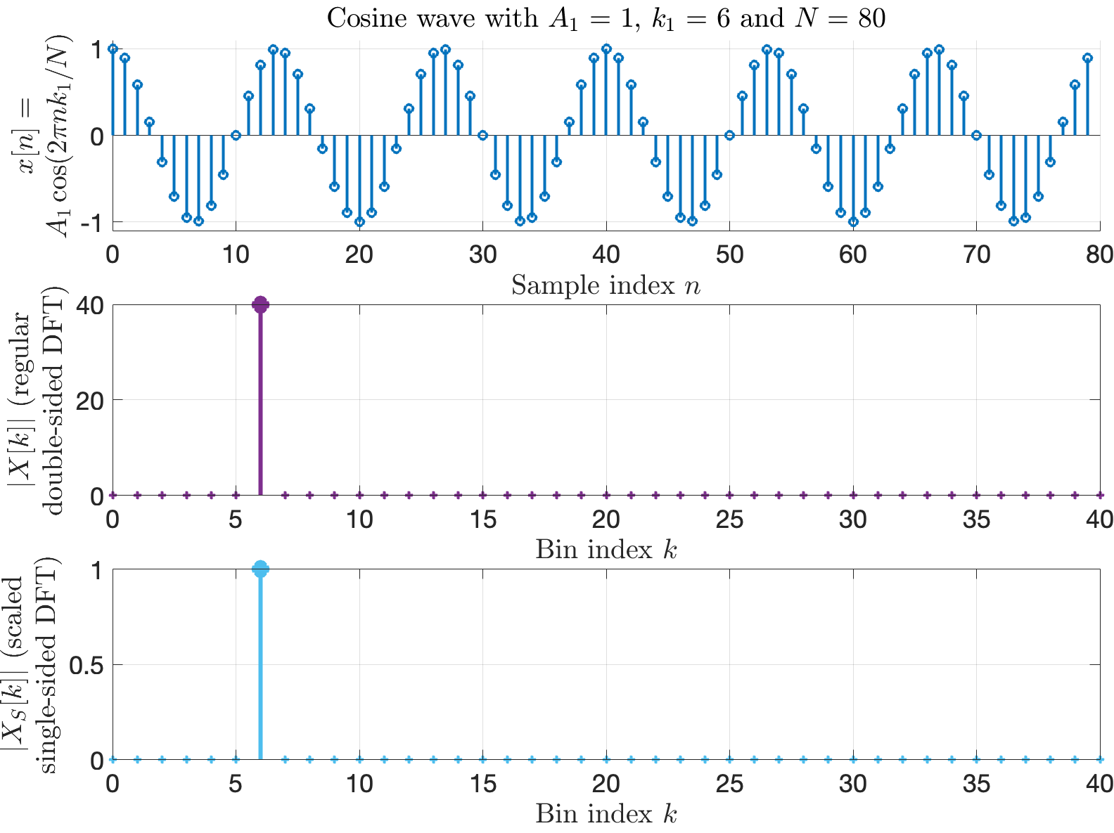**Figure 1:** Upper: The signal $x[n]$ from equation 7 plotted in the time domain. Centre: The regular double-sided DFT (via equation 2, with only the lower half of spectrum shown). Lower: The single-sided and scaled DFT (via equation 3).

Observations from Figure 1:

Upper: As expected, the time domain signal $x[n]$ has 80 samples in total, an amplitude of 1, and it completes 6 full cycles within the window of $N$ samples.
Centre: The regular DFT-computed frequency domain representation reveals a single non-zero complex amplitude, at bin index $k=6$ , of magnitude 40 (i.e., $\frac{N}{2}$ ). As expected, the frequency domain amplitude has accumulated a scaling factor that depends on $N$ . Only the lower half of the spectrum is shown (i.e., up to $k = \frac{N}{2}$ ), but we know from elsewhere that a conjugate copy of this lower half appears in the upper half of the spectrum, with another non-zero bin entry at $k = 80-6 = 74$ , also of magnitude $\frac{N}{2}$ .
Lower: The scaled DFT-computed frequency domain representation reveals a single non-zero complex amplitude, at bin index $k=6$ , of magnitude 1. In other words, this demonstrates that, under these idealised conditions, equation 5 is indeed satisfied. We therefore have an appropriate way to scale our DFT so its units match those of our time domain signal.

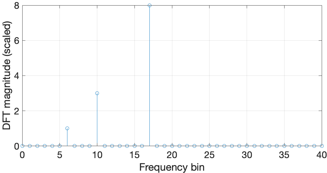
2.7 Example 2 – Signal with three periodic frequency components (+ Matlab code)

We can expand the previous example for a signal containing three frequency components that are periodic in $N$ samples. Code to illustrate this is shown below (note that the somewhat convoluted indexing in lines 6, 11, and 12 is to emphasise the difference between the usual DFT indexing of equation 2, which starts at 0, and what is required in Matlab, which starts at 1).

N       = 80;                       % Total number of samples
A1      = [1,3,8];                  % Signal amplitude (time domain)
k1      = [6;10;17];                % Signal frequency (time domain)

nVec    = 0:N-1;                    % Time index vector
kVec_SS = nVec((0:(N/2))+1);        % Single-sided frequency index vector

x       = A1*cos((2*pi*k1*nVec)./N);% Make a discrete time domain signal

x_dft   = fft(x);                   % Basic DFT of x
x_dft_S = x_dft((0:(N/2))+1);       % Single-sided DFT of x (even-length N)
x_dft_S((1:(N/2)-1)+1) = (2/N)*x_dft_S((1:(N/2)-1)+1); % Scaled single-sided DFT of x
x_dft_S(1)   = (1/N)*x_dft_S(1);    % Deal with DC
x_dft_S(end) = (1/N)*x_dft_S(end);  % Deal with Nyquist

stem(kVec_SS, abs(x_dft_S))
xlabel('Frequency bin')
ylabel('DFT magnitude (scaled)')

The result of the code above is shown in Figure 2.

**Figure 2:** The figure obtained by running the code in Example 2. Three discrete frequency components are clearly present, and their scaled DFT magnitudes match those of the original discrete time signal.

2.8 Example 3 – Cosine wave with linear ramping (i.e., a non-stationary signal)

Three important caveats about the use of DFT scaling were outlined above. In this example, we briefly illustrate the relevance of the second caveat, i.e., stationarity.

Consider a signal defined as

(8) $\begin{align*} x[n] = \frac{n}{N} A_1 \cos (2 \pi n k_{1}/N) \end{align*}$

which is the product of our original cosine wave (equation 1) and a linearly increasing ramp from 0:1.

The signal defined by equation 8 is interesting, because it seems to have only a single frequency component, but an evolving amplitude. Hence, it is not stationary, and there is no sense in which it has a single time domain amplitude. We would expect that scaling the complex amplitudes of its DFT in the frequency domain, via equation 3, will provide a similarly ambiguous result.

**Figure 3:** Upper: The signal $x[n]$ from equation 8 plotted in the time domain. Centre: The regular double-sided DFT (via equation 2, with only the lower half of spectrum shown). Lower: The single-sided and scaled DFT (via equation 3).

Analysis of this signal, following a similar structure to that of Example 1, is illustrated in Figure 3. We observe:

Upper: The linear ramp has an average value of 0.5.
Centre: The spectrum no longer has a single frequency component at $k=k_1$ , but instead all the bins have non-zero magnitudes. The signal energy in $x[n]$ is therefore spread across all frequencies.
Lower: The scaled DFT has $| X[k=k_1] | = 0.5$ , which is the same as the average value of the ramp. So in some sense the scaled DFT representation is still useful, in that it’s telling us something about the average value of the frequency component at $k_1$ , which does correspond with what we might expect from the time domain representation.However, because we know the `actual’ form of the time domain signal, via equation 8, we know that this does not correspond to a steady cosine wave. In real world measurements where we can’t be sure that the time domain signal is steady, care is needed in interpreting the scaled DFT.
Key message: Care is needed in how we interpret scaled DFT amplitudes, particularly when our time domain signal varies in amplitude over the course of the analysis window, and/or is not strictly periodic within the analysis window.

3 (In detail) Amplitude scaling in the time and frequency domains

3.1 Introduction

Having demonstrated the basic calculations required to produce a scaled version of the DFT, such that amplitude units in the time and frequency domains match each other (with caveats), in this section we will lay out some of the mathematical proofs that underpin this useful result.

3.2 DFT of a cosine signal that is periodic in $N$

Let’s start by evaluating the DFT of the pure cosine signal defined in equation 1, using equation 2 and Euler’s identity, to give

(9) $\begin{align*} X[k] &= \sum_{n=0}^{N-1} A_1 \cos{(2\pi n k_1 /N)} e^{-i 2 \pi k n /N}, \hspace{0.5cm} k = 0, 1, 2, ... , N-1 \\ &= \sum_{n=0}^{N-1} \frac{A_1}{2}(e^{i2\pi n k_1 /N} + e^{-i2\pi n k_1 /N}) e^{-i 2 \pi k n /N} \nonumber\\ &= \frac{A_1}{2}\left(\sum_{n=0}^{N-1} e^{i2\pi n k_1 /N} e^{-i 2 \pi k n /N} + \sum_{n=0}^{N-1}e^{-i2\pi n k_1 /N} e^{-i 2 \pi k n /N} \right) \nonumber\\ &= \frac{A_1}{2} \Biggl( \underbrace{{\sum_{n=0}^{N-1} {\underbrace{(e^{i 2\pi (k_1 - k) /N})}_{q}}}{^n}}_{Q_k} + \underbrace{{\sum_{n=0}^{N-1} {\underbrace{(e^{-i 2\pi (k_1 + k) /N})}_{r}}}{^n}}_{R_k} \Biggr) \nonumber\\ &= \frac{A_1}{2}\underbrace{\sum_{n=0}^{N-1} {q^n}}_{Q_k} + \frac{A_1}{2}\underbrace{\sum_{n=0}^{N-1}{r^n}}_{R_k} \nonumber\\ \rightarrow X[k] &= \frac{A_1}{2}Q_k + \frac{A_1}{2}R_k\nonumber \end{align*}$

Notice that in cases where either $q$ or $r$ evaluate to 1, the corresponding summation becomes a sum of 1, $N$ times over, which gives us $N$ .

Notice also that in cases where $q$ and $r$ are not equal to 1 (see here for details), we can re-express equation 9 as a closed form finite geometric series, to give

(10) $\begin{align*} X[k] &= \frac{A_1}{2} \Biggl(\underbrace{\left(\frac{1 - e^{i 2\pi (k_1 -k)}}{1 - e^{i 2\pi (k_1 -k)/N}}\right)}_{Q_k \text{ for } q\ne 1} + \underbrace{\left(\frac{1 - e^{-i 2\pi (k_1 +k)}}{1 - e^{-i 2\pi (k_1 + k)/N}}\right)}_{R_k \text{ for } r\ne 1} \Biggr) \end{align*}$

Equations 9 and 10 are very useful results, which will become clear when we consider what happens for particular values of $k_1$ and $k$ .

3.2.1 The case where $k=k_1$

Consider $k = k_1$ : Via equation 9, the exponent within $q$ becomes 0, and hence $q=1$ . By inspection we see that

(11) $\begin{align*} Q_{k_1} &= N \end{align*}$

Meanwhile, the exponent within $r$ is not 0 (nor is it an integer multiple of $i2\pi$ ), and hence $r\ne1$ . We therefore examine the corresponding expression for $R_k$ in equation 10, and see that the numerator evaluates to 0 (since $e^{-i 2\pi m} = 1$ for any integer $m$ ), and the denominator not to zero, and hence

(12) $\begin{align*} R_{k_1} &= 0 \end{align*}$

Via a similar argument, all terms of $X[k]$ , other than at $k=k_1$ , also evaluate to 0.

This leaves us with

(13) $\begin{align*} X[k={k_1}] &= \frac{A_1}{2} N \end{align*}$

from which we notice that the amplitude term $A_1$ has been scaled by a factor $\frac{N}{2}$ .

As expected, $X[k_1]$ is the `lower half’ of the cosine wave’s DFT representation. The factor of $\frac{1}{2}$ comes from the complex representation of a cosine wave as a pair of oppositely rotating complex phasors, and the $N$ factor from the DFT summation itself. Both of these will be `undone’ via appropriate re-scaling, summarised below.

3.2.2 The case where $k=N-k_1$

Consider $k = N-k_1$ : Via equation 9, the exponent in the $r$ term is $-i2\pi n$ , and hence $r=1$ (for any value of $n$ ). By inspection we see that

(14) $\begin{align*} R_{N-k_1} &= N \end{align*}$

Meanwhile, the exponent in the $q$ term is not 0 (nor is it an integer multiple of $i2\pi$ ), and hence $q\ne1$ . We therefore examine the corresponding expression for $Q_k$ in equation 10, and see that the numerator evaluates to 0 (since $e^{-i 2\pi m} = 0$ for any integer $m$ ), and the denominator not to zero, and hence

(15) $\begin{align*} Q_{N- k_1} &= 0 \end{align*}$

Via a similar argument, all terms of $X[k]$ , other than at $k=k_1$ , also evaluate to 0.

This leaves us with

(16) $\begin{align*} X[k={N-k_1}] &= \frac{A_1}{2} N \end{align*}$

Similar comments can be made about the meaning of $X[N-k_1]$ as those the preceding sub-section.

3.2.3 Special case where $k_1=0$

Consider $k = 0$ : If we go back to our original DFT of equation 2, a few steps of algebra reveal that

(17) $\begin{align*} X[0] &= \sum_{n=0}^{N-1} x[n] e^{0}\\ &= \sum_{n=0}^{N-1} x[n]\nonumber \end{align*}$

The entry at $X[0]$ is often called as the `DC’ bin, and is formed by adding together all the samples in $x[n]$ . It is also purely real, for a real-valued $x[n]$ , and appears only once in the spectrum. %Unlike the entries for $k\ne0$ , there is no constant scaling factor by $N$

For the signal $x[n]$ of equation 1, which is perfectly periodic in $N$ samples, it is both intuitively clear, and quite straightforward to demonstrate, that if $k_1\ne0$ , the sum of all samples of $x[n]$ will evaluate to 0.

In the specific case where $k_1 = 0$ , our signal $x[n]$ becomes the unit step, scaled by $A_1$ . Therefore equation 17 becomes

(18) $\begin{align*} X[0] &= \sum_{n=0}^{N-1} A_1\\ &= A_1\sum_{n=0}^{N-1} 1\nonumber \\ \rightarrow X[0] &= A_1 N \end{align*}$

By inspection we see that the average value of $x[n]$ must be $A_1$ , and an appropriate scaling of the DFT to match this at $k=0$ is given by

(19) $\begin{align*} X_S[0] &= \left(\frac{1}{N}\right) \cdot X[0] \end{align*}$

3.2.4 Special case where $k_1=\frac{N}{2}$

Consider $k = \frac{N}{2}$ : Again returning to our original DFT of equation 2, a few steps of algebra reveal that

(20) $\begin{align*} X[0] &= \sum_{n=0}^{N-1} x[n] e^{-i\pi n}\\ &= \sum_{n=0}^{N-1} x[n] (-1)^n \nonumber \end{align*}$

since $e^{-i\pi} = -1$ .

This is interesting since, as with $X[0]$ , $X[\frac{N}{2}]$ is always purely real. It is also unique, without a separate `lower half’ and `upper half’ representation across the analysis bandwidth.

If $k_1\ne N/2$ , we know via equations 12 and 15 that

(21) $\begin{align*} X\left[ \frac{N}{2} \right] &= 0 \end{align*}$

However, if $k_1 = \frac{N}{2}$ , via equation 9 we obtain

(22) $\begin{align*} X\left[\frac{N}{2} \right] &= \frac{A_1}{2} \left( \sum_{n=0}^{N-1} e^{i\pi n} e^{-i\pi n} + \sum_{n=0}^{N-1} e^{-i\pi n} e^{-i\pi n} \right)\\ &= \frac{A_1}{2} \left( \sum_{0}^{N-1} e^0 + \sum_{0}^{N-1} e^{-i2\pi n} \right) \nonumber\\ &= \frac{A_1}{2} N + \frac{A_1}{2} N\nonumber \\ \rightarrow X\left[\frac{N}{2} \right] &= A_1N \end{align*}$

Therefore, as with the $k_1=0$ case, appropriate scaling of $X\left[\frac{N}{2} \right ]$ is achieved via

(23) $\begin{align*} X_S\left[ \frac{N}{2} \right] &= \left(\frac{1}{N}\right) \cdot X\left[ \frac{N}{2} \right] \end{align*}$

3.3 Summary

Pulling together all of the above, for a single frequency cosine signal $x[n]$ of amplitude $A_1$ , integer frequency $k_1$ , and sampled over $N$ samples:

For $k \ne [0, \frac{N}{2}]$ : The DFT, $X[k]$ , has amplitude $\frac{A_1}{2} N$ at each of $k=k_1$ (`lower half’) and $k=N-k_1$ (`upper half’). If we want a single-sided spectrum representation $X_{S}[k]$ (i.e., $k \in [0:\frac{N}{2}]$ ) with spectral amplitudes that match $x[n]$ (i.e., $A_1$ ), we therefore need to scale $X[k]$ via

(24) $\begin{align*} X_S[k] = \left(\frac{2}{N} \right)\cdot X[k] \end{align*}$

For $k = [0, \frac{N}{2}]$ : The DFT, $X[k]$ , has a single complex amplitude of value $A_1 N$ . For these bins only, our scaled DFT is therefore obtained via

(25) $\begin{align*} X_S\left[0\right] &= \left(\frac{1}{N} \right)\cdot X\left[0\right] \\ X_S\left[\frac{N}{2}\right] &= \left(\frac{1}{N} \right)\cdot X\left[\frac{N}{2}\right] \end{align*}$

At last, these expressions provide the DFT scaling condition given at the start in equation 3, in cases where $N$ is even.

In cases where $N$ is odd, there is no bin entry at exactly $\frac{N}{2}$ , so we don’t need a special scaling there. The rest of the arguments can be translated quite straightforwardly from the case where $N$ is even.

4 Amplitude scaling for periodic signals with a constant phase shift

What happens to the results in the preceding section if we introduce a phase shift $\phi$ to the discrete time signal, and instead analyse this new signal $x^{ps}[n]$ defined as

(26) $\begin{align*} x^{ps}[n] = A_1 \cos \left(\frac{2 \pi n k_{1}}{N} + \phi\right) \end{align*}$

Following the same analysis, but skipping most of the steps, it is possible to show, via a similar argument to that in equation 9, that

(27) $\begin{align*} X^{ps}[k] &= \frac{A_1 e^{i\phi}}{2}Q_k + \frac{A_1 e^{-i\phi}}{2}R_k \end{align*}$

where $Q_k$ and $R_k$ are defined exactly as in equation 9.

Equation 27 reveals a pair of complex-valued spectral amplitudes, which we know via the Hermitian symmetry property of the DFT to be the conjugates of each other. Following a similar analysis to that above, at $k=k_1$ we have

(28) $\begin{align*} X^{ps}[k=k_1] = \frac{A_1 e^{i\phi}}{2} N \end{align*}$

Via the multiplicative property of complex numbers (magnitude of a product is the product of the magnitudes), the magnitude is given by

(29) $\begin{align*} |X^{ps}[k_1]| = \left|\frac{A_1 N}{2}\right| \left|e^{i\phi}\right| = \left|\frac{A_1 N}{2}\right| \end{align*}$

since $|e^{i\phi}| = 1$ for any constant $\phi$ . Clearly, scaling this result requires the same computations as previously.

In other words, whatever the initial phase of the discrete time signal, the DFT amplitude scaling approach can be applied in the same way. However, in general it should be applied to the magnitude of the (complex valued) spectral amplitudes.

5 Power spectra

To be added.

6 Further reading

[1] Jens Ahrens et al (2020). Tutorial on Scaling of the Discrete Fourier Transform and the Implied Physical Units of the Spectra of Time-Discrete Signals. Audio Engineering Society Convention e-Brief 600, 2020.

https://appliedacousticschalmers.github.io/scaling-of-the-dft/

[2] Mathworks: Amplitude Estimation and Zero Padding

https://uk.mathworks.com/help/signal/ug/amplitude-estimation-and-zero-padding.html

[3] Mathworks: Webinar on Understanding Power Spectral Density and the Power Spectrum

https://uk.mathworks.com/videos/understanding-power-spectral-density-and-the-power-spectrum-1707740400025.html

Contents