The Discrete Fourier Transform: Useful maths

Introduction
Vectors in 3D real space
Discrete time signals as N-length complex valued vectors
Geometric sequences and discrete time signals
Sine waves from complex phasors
Geometric series

1 Introduction

A handful of mathematical tools are particularly useful in understanding the structure and use of the Discrete Fourier Transform (DFT). Several of them are gathered together here on a single page.

The other pages within the signals and signal processing section use this page as essential background.

2 Vectors in 3D real space

2.1 Introduction

It can be useful to treat discrete time signals, such as sampled audio signals stored in computer memory, as `vectors’ of numbers. Indeed, much of DSP is based upon the mathematical tools of vectors and Euclidian geometry (sines, cosines, phase angles, $\pi$ , etc).

We begin this page with a quick overview of key metrics used to describe vectors in 3D real space, which will be extended below to arbitrary length discrete time signals.

2.2 The dot product as an inner product

In regular 3D real space, the inner product $q$ , between two vectors $\underline{a}$ and $\underline{b}$ , is equivalent to the dot product. It can therefore be obtained by multiplying the lengths of the two vectors together with the cosine of the angle between them

(1) $\begin{align*} q = \langle \underline{a}, \underline{b} \rangle = \underline{a}\cdot\underline{b} = |{a}| |b| \cos{(\theta)} \end{align*}$

where | ${a}$ | means the Euclidian length of $\underline{a}$ (also referred to as the magnitude of $\underline{a}$ ).

Evaluating $q$ via equation 1 will return a scalar number, which will be 0 if the vectors are orthogonal, and nonzero otherwise.

In somewhat loose language, $q$ tells us something about how much $\underline{a}$ `overlaps’ $\underline{b}$ , and vice versa (since it can be shown that $\langle \underline{a}, \underline{b} \rangle = \langle \underline{b}, \underline{a} \rangle$ ).

2.3 Vector norm and length

If we take the inner product of the vector $\underline{a}$ with itself, we obtain

(2) $\begin{align*} \langle \underline{a}, \underline{a} \rangle = \underline{a}\cdot\underline{a} = |{a}| |{a}| \cos{(0)} = |a|^2 \end{align*}$

from which it can be seen by inspection that the `length’ of overlap of $\underline{a}$ with itself, i.e., its effective length regardless of direction, is given by

(3) $\begin{align*} \sqrt{\langle \underline{a}, \underline{a} \rangle} = |a| \end{align*}$

which is another way of saying that the length of $a$ is the magnitude of $a$ (i.e., $|a|$ ).

The quantity $\sqrt{\langle \underline{a}, \underline{a} \rangle}$ is known as the norm of $\underline{a}$ , which for a vector in 3D real space also corresponds to its length (or indeed, magnitude).

3 Discrete time signals as N-length complex valued vectors

3.1 Introduction

Consider $N$ -length complex valued discrete time signals, say $u=u[n]$ and $v=v[n]$ , specified at integer sample time indices $n$ (the sample rate is not important here). Each signal comprises $N$ samples, and therefore runs from $n = 0, 1, 2, \cdots, N-1$ .

The signals $u, v$ can be viewed as a pair of $N$ -dimensional vectors in $\mathbb{C}_N$ space (i.e., each vector has $N$ numbers, each of which is, in general, complex valued).

3.2 Inner product for discrete time signals

The inner product between $u$ and $v$ , which we’ll call $q$ , is obtained via

(4) $\begin{align*} q = \langle u, v \rangle = \sum_{n=0}^{N-1} u[n] v^{\ast}[n] \end{align*}$

where $^{\ast}$ denotes the complex conjugate. As with the real space dot product, extension of the inner product to $u, v \in \mathbb{C}_N$ renders a scalar $q$ that tells us about the `amount of overlap’ between the signals (albeit that $q$ will be complex valued, in general).

Fourier analysis, including the Discrete Fourier Transform, is about examining the `amount of’ a given frequency component within a given signal, so it is not hard to imagine that the inner product may be a useful tool, in due course.

3.3 Discrete time signal energy

If we take the inner product of the signal $u$ with itself, we obtain

(5) $\begin{align*} \langle u, u \rangle &= \sum_{n=0}^{N-1} u[n] u^{\ast}[n] = \sum_{n=0}^{N-1} |u[n]|^{2} \\ &= \|{u}\|^2 \end{align*}$

The quantity $\|{u}\|^2$ is sometimes referred to as the `total energy’ of the signal, though care is needed in this interpretation, particularly when comparing time domain and frequency domain signal metrics.

It’s also sometimes called the `squared L2 norm’. Notice the conceptual similarity with the real space example in equation 2 above.

3.4 Discrete time signal length and the L2-norm

Analogous with the real space example of equation 3, an $N$ -length complex valued discrete signal, $u[n]$ , can be thought of as having an $N$ -dimensional `length’. This is usually defined in terms of the L2-norm (aka Euclidian norm), $\|{u}\|$ , as

(6) $\begin{align*} \|{u}\| &= \sqrt{\langle u, u \rangle} = \sqrt{\sum_{n=0}^{N-1} |u[n]|^{2}} \\ &= \sqrt{\|{u}\|^2} \end{align*}$

using the definition in equation 5. Sometimes $\|{u}\|$ is written as $\|{u}\|_{2}$ (where the 2 is a subscript, not a superscript), to be explicit that it is the L2-norm, but in general where $\|{u}\|$ is written we assume reference to the L2-norm.

Later on we will see how useful it is to have strict definitions of `energy’ and `length’ when it comes to comparing the units of signals expressed in the discrete time vs. discrete frequency domains.

4 Geometric sequences and discrete time signals

4.1 Geometric sequences

Consider an arbitrary number $z_{1} \in \mathbb{C}$ , i.e., a complex valued number with a real and an imaginary part (say, $z_{1} = a + i b$ where $i = \sqrt{-1}$ , and $a, b$ are real valued numbers).

In DSP it is often helpful to define special signals that are expressed as a geometric sequence based upon a single complex number. For example, we might define a discrete time signal $x[n]$ as

(7) $\begin{align*} x[n] = (z_{1})^{n} \end{align*}$

where $n$ takes on integer values between 0 and $N-1$ , i.e., $n\in 0:N-1$ .

The signal $x[n]$ describes a `finite geometric sequence’, where each entry comes from raising the number $z_{1}$ to an integer power $n$ .

4.2 Geometric sequence: Example

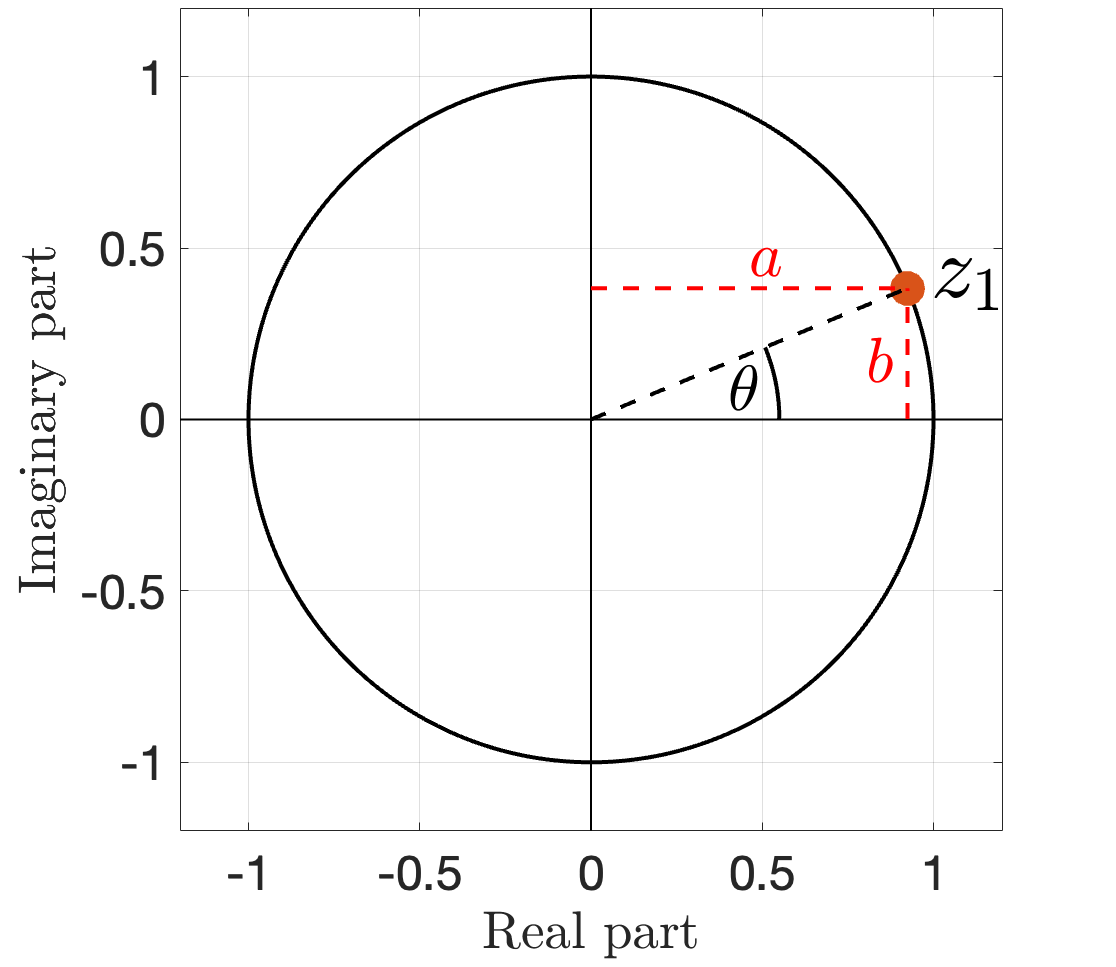
As an example, consider the complex number

(8) $\begin{align*} z_{1} = e^{\frac{i 2\pi}{16}} \end{align*}$

which describes a single point on the complex plane, illustrated in Figure 1.

**Figure 1:** A single complex number $z_1$ shown as an orange point on the complex plane.

As with any single complex number, $z_1$ can be parameterised by the angle it makes from the positive real axis, $\theta$ (which is $2\pi/16$ in this case), and its distance from the origin (1, in this case). It can also be parameterised in terms of its separate real and imaginary parts. In other words

(9) $\begin{align*} z_{1} = e^{\frac{i 2\pi}{16}} = a + ib \end{align*}$

which are labelled in Figure 1.

We can use $z_1$ to generate a periodic sequence of numbers by inserting it into equation 7, to produce

(10) $\begin{align*} x[n] = (z_{1})^{n} = (e^{\frac{i 2\pi}{16}})^n = e^{\frac{i 2\pi n}{16}} \\ \text{for} \hspace{0.2cm} n &= 0, 1, 2, ... , N-1 \nonumber \\ \text{i.e., for} \hspace{0.2cm} n &= 0, 1, 2, ... , 15 \nonumber \end{align*}$

since in this case we have defined $N = 16$ , and there are therefore exactly 16 entries in $x[n]$ .

It is instructive to examine how the entries in $x[n]$ , as defined in equation 10, change with each new value of $n$ . Here are the first few values:

(11) $\begin{align*} n &=0 \rightarrow x[0] = e^{0} = 1\\\nonumber n &=1 \rightarrow x[1] = e^{\frac{i 2\pi}{16}}\\\nonumber n &=2 \rightarrow x[2] = e^{\frac{i 4\pi}{16}}\\\nonumber n &=3 \rightarrow x[3] = e^{\frac{i 6\pi}{16}}\\\nonumber \end{align*}$

and all 16 values are plotted on the complex plane in Figure 2.

**Figure 2:** All 16 entries in the signal $x[n]$ defined in equation 10 shown as orange points on the complex plane. The numbers indicate the corresponding value of $n$ for each point in the sequence.

Starting at $n=0$ we see that $x[0]$ takes the value 1, and hence this point lies at a distance of 1 away from the origin along the real axis.
For $n=1$ , $x[1]$ is just our original complex number, $z_1$ , as marked on Figure 1 (the dashed line in Figure 2 is the same as that shown in Figure 1, to emphasise this point).
For $n=2$ , $x[2]$ `jumps’ anticlockwise from where it was at $n=1$ , tracing out another $\theta$ radians in the process.For $n=3$ , $x[3]$ `jumps’ another $\theta$ radians, anticlockwise, from where it was at $n=2$ .
As $n$ increments towards $n=15$ , we see that it traces out a series of points that lie along a circle of radius 1, centred at the origin. This special circle is known as the `unit circle’, and is marked in black on Figure 2. It has importance across DSP, well beyond the generation of periodic signals.

In other words, $x[n]$ describes a sampled phasor, of magnitude 1, rotating anticlockwise on the complex plane.

Note that if we were to examine $n=16$ , which would correspond to the 17th consecutive value of $n$ , we would find that $x[16]$ takes on exactly the same value as it did for $n=0$ . We therefore see that the $x[n]$ defined in equation 10 is periodic, with a period of exactly 16 samples, since calculating entries for values of $n>15$ simply `plays back’ the same sequence of numbers calculated in the range $n\ = 0, 1, 2 ... 15$ .

4.3 Roots of unity

The 16 values of $x[n]$ calculated via equation 10 are sometimes referred to as the `roots of unity’. In this case, because of the way we defined $x[n]$ , there are exactly 16 of them.

Changing the value of $N$ to, say, 20, would result in a sampled phasor with 20 unique sample locations, and therefore expressing 20 roots of unity.

In general, a signal $x[n]$ defined via

(12) $\begin{align*} x[n] = e^{\frac{i 2\pi n}{N}} \\ \text{for} \hspace{0.2cm} n &= 0, 1, 2, ... , N-1 \nonumber \end{align*}$

will express the $N$ roots of unity, since raising any of the entries in $x[n]$ to the power $N$ will result in

(13) $\begin{align*} x[n] = (e^{\frac{i 2\pi n}{N}})^N = e^{i2\pi n} = 1 \end{align*}$

for any integer value of $n$ .

Graphically, it is clear from Figure 2 that the sequence $x[n]$ , as defined in equation 12, divides the unit circle into $N$ `slices’ of equal angular spacing.

5 Sine waves from complex phasors

Although the sampled complex phasor defined in equation 12 seems `complicated’, due to its use of complex numbers, it should be clear from the preceding sections that the mathematics are actually quite simple. This is because complex exponential arithmetic is generally straightforward, particularly in the context of DSP.

Indeed, this is an illustrative example of why is can be useful to undertake certain tasks with a particular representation, even if later converting to a different representation — we’ll see more of this when examining time domain and frequency domain signal representations.

It is natural to ponder whether such expressions are useful in the `real world’. One way to address this is to re-express equation 12 via Euler’s identity, and then take, for example, only the imaginary part ( $\Im$ ), to generate a new discrete time signal $y[n]$ . We can formalise this via

(14) $\begin{align*} y[n] &= \Im \left[ e^{\frac{i 2\pi n}{N}} \right]\\ &= \Im \left[ \cos{\left( \frac{2\pi n}{N} \right)} + i \sin{\left( \frac{2\pi n}{N} \right)} \right]\nonumber\\ &= \sin{\left( \frac{2\pi n}{N} \right)} \nonumber \end{align*}$

which demonstrates that taking the imaginary part of the sampled complex phasor will create a sampled sine wave.

Figure 3 illustrates the creation of a sampled sine wave from a sampled complex phasor, via equation 14.

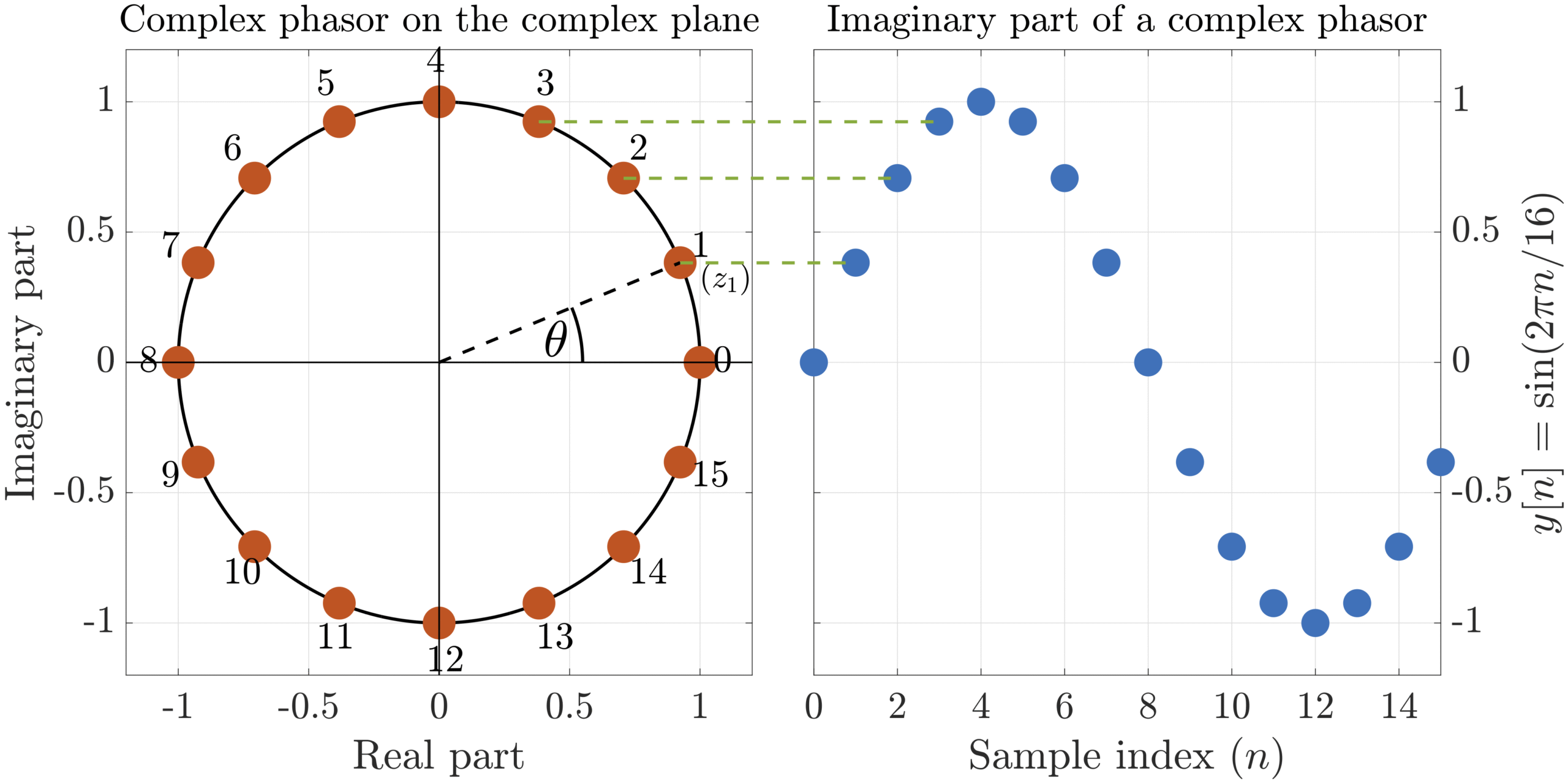
**Figure 3:** Creation of a sampled sine wave from equation 14 with $N=16$ . The signal $y[n]$ is defined as the imaginary part (only) of a complex phasor. The green dashed lines illustrate the correspondence between phasor values and sine values for $n = 2$ and $3$ .

6 Geometric series

Adding together all numbers in the geometric sequence defined in equation 7, from $n = 1$ up to $n=N-1$ , is known as a finite geometric series, and may be written

(15) $\begin{align*} \sum_{n=0}^{N-1}x[n] = \sum_{n=0}^{N-1}(z_{1})^{n}. \end{align*}$

If $z_{1}=1$ (i.e., $z_{1}$ is purely real and of value 1), then equation 15 simply reduces to a sum of $N$ values of 1, such that

(16) $\begin{align*} \sum_{n=0}^{N-1}(1)^{n} = N. \end{align*}$

Crucially, it can be shown that if $z_{1} \ne 1$ , equation 15 may instead be expressed as

(17) $\begin{align*} \sum_{n=0}^{N-1}(z_{1})^{n} = \frac{1-(z_{1})^N}{1-z_{1}}. \end{align*}$

which turns out to be very useful in demonstrating key properties of the Discrete Fourier Transform (DFT), amongst other things.

It’s useful because we now have a simple way to add up the values of a finite length discrete time signal, and indeed the product of disctete time signals, whatever the value of the signal.

Contents